
今天给大家介绍的是BMKMANU S1000空间转录组数据与单细胞转录组数据的关联分析。在我们的关联分析中可以使用不同分辨率的空间数据分别与单细胞数据进行关联分析,本次我们使用spatialDWLS进行100μm关联分析,下周我们则会推出多级分辨率下的关联分析。详细分析流程如下所示:
spatialDWLS
spatialDWLS首先使用细胞类型富集分析方法来确定哪些类型的细胞在每个位置具有较高的概率,然后使用阻尼加权最小二乘法(DWLS)的扩展来确定指定位置的细胞类型的组成。与现有的去卷积方法相比,关键区别在于SpatialDWLS包含额外的过滤步骤,以去除不相关的细胞类型,从而增强特异性。
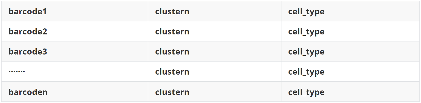
1、单细胞数据格式要求
(1)data 1 聚类和注释结果(sc_meta.txt)
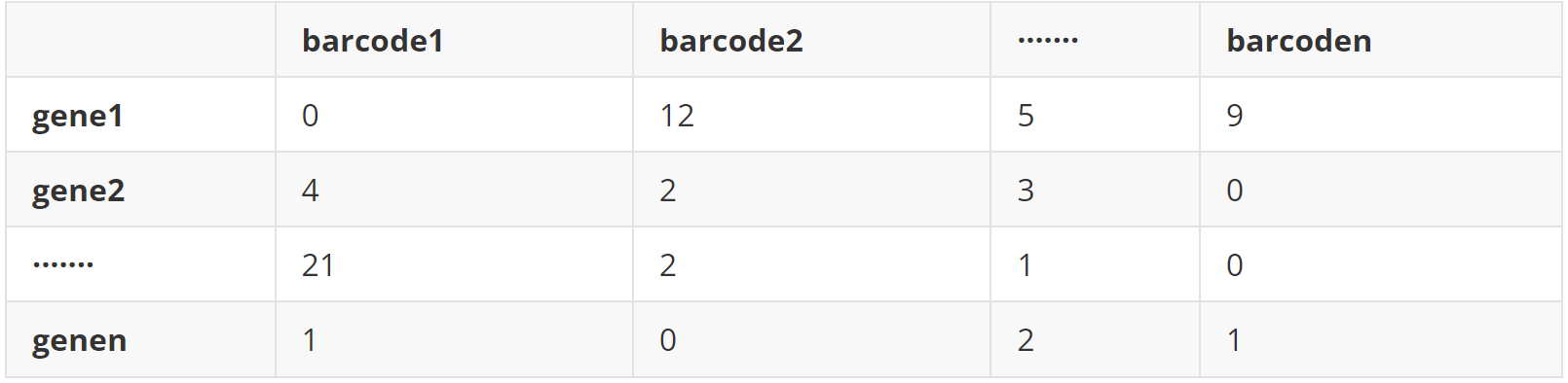
 (2)data 2 基因表达矩阵(all_cells_count_matrix_filtered.tsv)
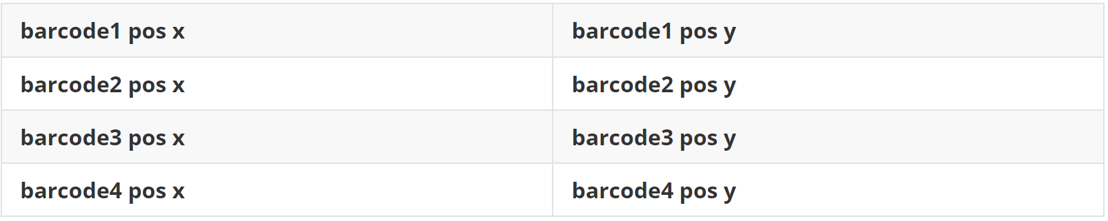
2、空间数据格式要求
(1)data 1 空间spots位置文件(loc.txt)
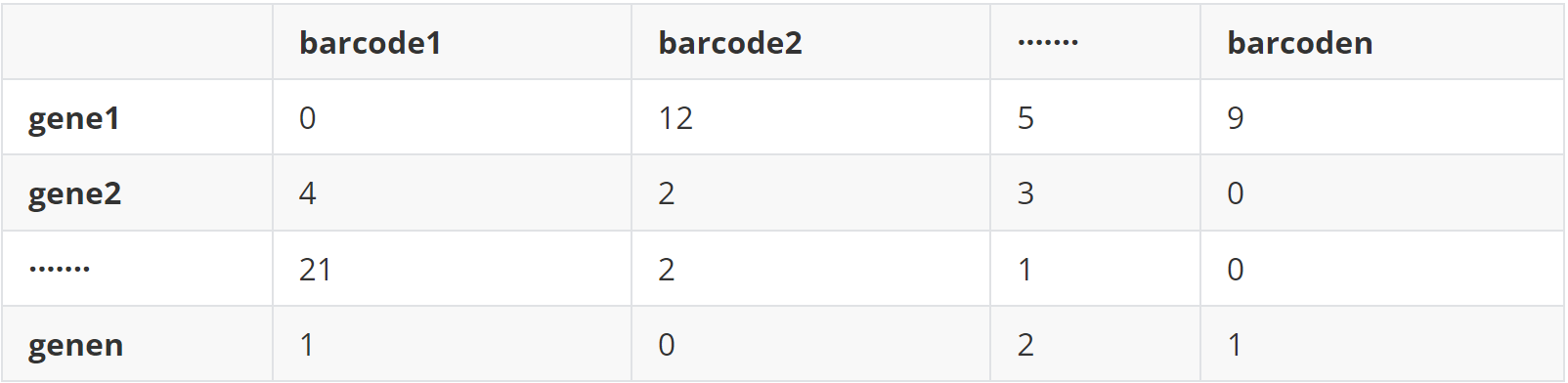
(2)data 2 基因表达矩阵(exp.txt)
 #安装Giotto
library(devtools) # if not installed: install.packages(‘devtools’)
library(remotes) # if not installed: install.packages(‘remotes’)
remotes::install_github(“RubD/Giotto”)
#加载R包
library(Seurat)
library(SingleR)
library(celldex)
library(Giotto)
library(ggplot2)
library(scatterpie)
library(data.table)
library(tibble)
#单细胞数据分析
#读入单细胞数据
sc_meta<-read.table(“../sc_meta.txt”,header = F,row.names = 1,sep=”\t”)
sc_data<-read.table(“../all_cells_count_matrix_filtered.tsv”,header = T,row.names = 1)
#设置python路径
my_python_path = “/xxx/software/miniconda3/bin/python”
instrs = createGiottoInstructions(python_path = my_python_path)
#创建Giotto 对象
sc <- createGiottoObject(raw_exprs = sc_data,instructions = instrs)
#表达数据标准分析
sc <- normalizeGiotto(gobject = sc, scalefactor = 6000, verbose = T)
sc <- calculateHVG(gobject = sc, save_plot = TRUE,save_param=list(save_name=”sc_HVGplot”))
gene_metadata = fDataDT(sc)
featgenes = gene_metadata[hvg == ‘yes’]$gene_ID
sc <- runPCA(gobject = sc, genes_to_use = featgenes, scale_unit = F)
signPCA(sc, genes_to_use = featgenes, scale_unit = F, save_plot = TRUE, save_param=list(save_name=”sc_signPCAplot”))
#使用Giotto中的DEG函数计算用于去卷积的Sig
sc@cell_metadata$leiden_clus <- as.character(sc_meta$V3)
scran_markers_subclusters = findMarkers_one_vs_all(gobject = sc,
method = ‘scran’,
expression_values = ‘normalized’,
cluster_column = ‘leiden_clus’)
Sig_scran <- unique(scran_markers_subclusters$genes[which(scran_markers_subclusters$ranking <= 100)])
#计算每种细胞类型中特征基因的表达中值
norm_exp<-2^(sc@norm_expr)-1
id<-sc@cell_metadata$leiden_clus
ExprSubset<-norm_exp[Sig_scran,]
Sig_exp<-NULL
for (i in unique(id)){
Sig_exp<-cbind(Sig_exp,(apply(ExprSubset,1,function(y) mean(y[which(id==i)]))))
}
colnames(Sig_exp)<-unique(id)
#空间数据分析
#读入数据
spatial_loc<-read.table(file=”loc.txt”,header = F)
spatial_exp<-read.table(file=”exp.txt”,header = T,row.names = 1)
#创建Giotto对象
st <- createGiottoObject(raw_exprs = spatial_exp,spatial_locs = spatial_loc,
instructions = instrs)
#对空间数据进行过滤,均一化和聚类
st <- filterGiotto(gobject = st,
expression_threshold = 1,
gene_det_in_min_cells = 5,
min_det_genes_per_cell = 100,
expression_values = c(‘raw’),
verbose = T)
st <- normalizeGiotto(gobject = st)
st <- calculateHVG(gobject = st, save_plot = TRUE, save_param=list(save_name=”st_HVGplot”))
gene_metadata = fDataDT(st)
featgenes = gene_metadata[hvg == ‘yes’]$gene_ID
st <- runPCA(gobject = st, genes_to_use = featgenes, scale_unit = F)
signPCA(st, genes_to_use = featgenes, scale_unit = F, save_plot = TRUE,save_param=list(save_name=”st_signPCAplot”))
st <- createNearestNetwork(gobject = st, dimensions_to_use = 1:10, k = 10)
st <- doLeidenCluster(gobject = st, resolution = 0.5, n_iterations = 1000)
#基于单细胞数据的基因表达特征和空间数据的Giotto对象进行去卷积分析
st <- runDWLSDeconv(gobject = st, sign_matrix = Sig_exp)
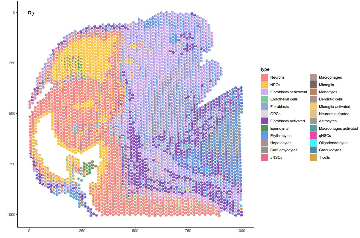
#可视化展示
plot_data <- as.data.frame(st@spatial_enrichment$DWLS)[-1]
plot_col <- colnames(plot_data)
plot_data$x <- as.numeric(as.character(st@spatial_locs$sdimx))
plot_data$y <- as.numeric(as.character(st@spatial_locs$sdimy))
min_x <- min(plot_data$x)
plot_data$radius <- 7
df <- data.frame()
p <- ggplot(df) + geom_point() + xlim(min(plot_data$x)-7, max(plot_data$x)+7) + ylim(min(plot_data$y)-7, max(plot_data$y)+7)
p <- p + geom_scatterpie(aes(x=x, y=y, r=radius), data=plot_data, cols=plot_col, color=NA, alpha=.8) +scale_y_reverse()+
geom_scatterpie_legend(plot_data$radius, x=1, y=1) +
scale_fill_manual(values = c(“#F56867″,”#FEB915″,”#C798EE”,”#59BE86″,”#7495D3″,”#D1D1D1″,”#6D1A9C”,”#15821E”,”#3A84E6″,”#997273″,”#787878″,”#DB4C6C”,”#9E7A7A”,”#554236″))+
theme_classic()
ggsave(p, filename = “plot.pdf”,height=8,width=5)


 京公网安备 11011302003368号