

- Open the script file
“`markdown
source(‘xxx’) # ‘xxx’ script path, for example ‘C:/Users/R/Desktop/qq.R’
“`
- Create a Seurat object and generate a spatial clustering plot
– `FilePath`: Directory path containing “barcode.tsv.gz, barcode_pos.tsv.gz, feature.tsv.gz, matrix.mtx.gz” files.
– `barcode_pos_file`: File path for “barcode_pos.tsv.gz.”
– `out_path`: Output directory.
– `png_path`: H&E staining image (.png format). If using .tiff format, make sure to convert it, and consider reducing the resolution during conversion to avoid large .png files that may fail to load. Note that the Seurat object’s name must be “object.”
“`R
object <- Create_object(
FilePath = ‘E:/AAAWork/BSTViewer_project/subdata/L13_heAuto/’,
barcode_pos_file = ‘E:/AAAWork/BSTViewer_project/subdata/L13_heAuto/barcodes_pos.tsv.gz’,
out_path = ‘C:/Users/R/Desktop/temp/Cluster/’,
png_path = ‘C:/Users/R/Desktop/temp/he.png’,
min.cells = 10, # Minimum cells for a gene to be retained, adjustable (default: 10).
min.features = 100, # Minimum features for a cell to be retained, adjustable (default: 100).
dims = 1:30, # Number of principal components for subsequent analysis, adjustable (default: 1:30).
resolution = 0.5, # Set the granularity for downstream analysis, higher values yield more clusters, adjustable (default: 0.5).
point_size = 3, # Point size, adjustable based on matrix file level (smaller level requires smaller values).
width = 12, # Output image width, adjustable (default: 12).
height = 5, # Output image height, adjustable (default: 5).
Cluster = T, # Perform clustering analysis (default: False).
label = T # Output clustered image with labels (default: True).
)
“`
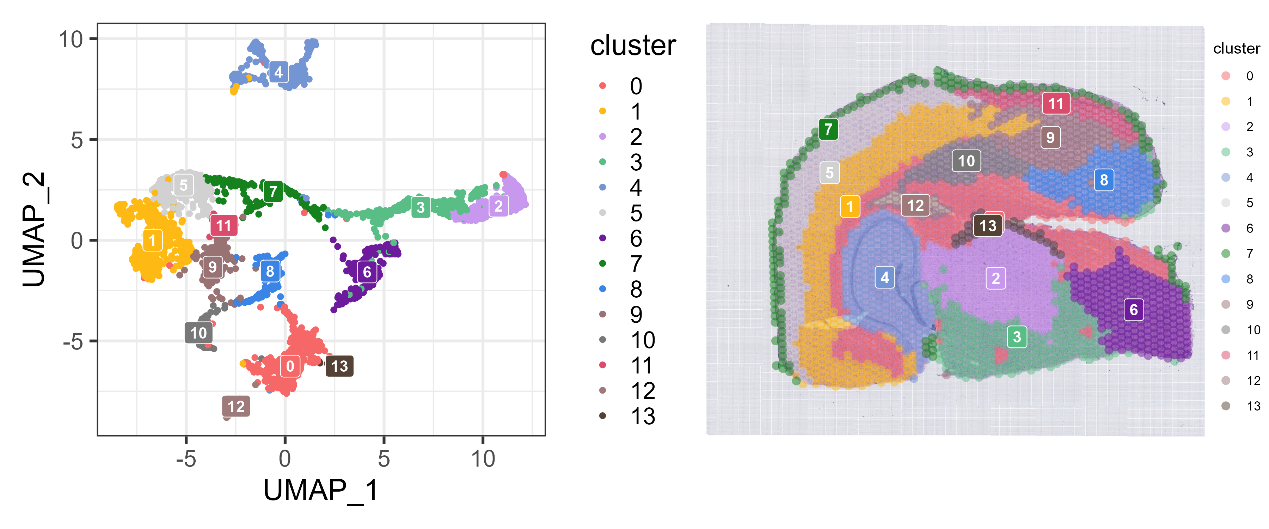
umap_cluster_label
- UMI Statistics
“`R
object <- Create_object(
FilePath = ‘E:/AAAWork/BSTViewer_project/subdata/L13_heAuto/’,
barcode_pos_file = ‘E:/AAAWork/BSTViewer_project/subdata/L13_heAuto/barcodes_pos.tsv.gz’,
out_path = ‘C:/Users/R/Desktop/temp/UMI_stat/’,
png_path = ‘C:/Users/R/Desktop/temp/he.png’,
point_size = 3, # Same as above.
width = 12, # Same as above.
height = 5, # Same as above.
UMI_stat = T # Whether to perform UMI statistics (default: True).
)
“`
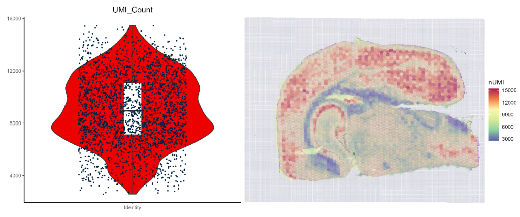
UMI_viol_heatmap
- nFeature Statistics
“`R
object <- Create_object(
FilePath = ‘E:/AAAWork/BSTViewer_project/subdata/L13_heAuto/’,
barcode_pos_file = ‘E:/AAAWork/BSTViewer_project/subdata/L13_heAuto/barcodes_pos.tsv.gz’,
out_path = ‘C:/Users/R/Desktop/temp/Gene_stat/’,
png_path = ‘C:/Users/R/Desktop/temp/he.png’,
point_size = 2, # Same as above.
width = 12, # Same as above.
height = 5, # Same as above.
nFeature_stat = T # Whether to perform nFeature statistics (default: True).
)
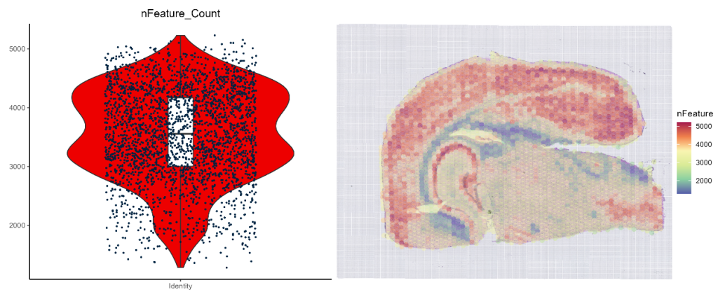
nFeature_viol_heatmap
- Output Marker Genes for Each Cluster and Create Expression Heatmaps for Single Genes
“`R
object <- Create_object(
FilePath = ‘E:/AAAWork/BSTViewer_project/subdata/L13_heAuto/’,
barcode_pos_file = ‘E:/AAAWork/BSTViewer_project/subdata/L13_heAuto/barcodes_pos.tsv.gz’,
out_path = ‘C:/Users/R/Desktop/temp/Single_gene_1/’,
png_path = ‘C:/Users/R/Desktop/temp/he.png’,
point_size = 2, # Same as above.
Gene_stat = T, # Whether to generate marker gene plots (default: False).
top_gene = 1, # Number of top marker genes to select for each cluster, adjustable (default: 1).
min.pct = 0.25, # Minimum percentage of a gene’s presence in any two cell groups, adjustable (default: 0.25).
logfc.threshold = 0.25, # Log-fold change threshold, adjustable (default: 0.25).
markpic_width = 8, # Width of violin and tsne plots, adjustable.
markpic_height = 12 # Height of violin and tsne plots, adjustable.
)“`
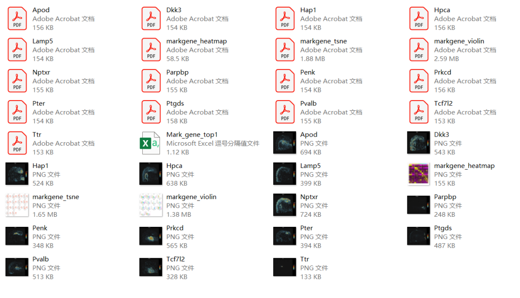
Heatmaps list
- Generate Cluster Plots for Specific Gene(s)
“`R
object <- Create_object(
FilePath = ‘E:/AAAWork/BSTViewer_project/subdata/L13_heAuto/’,
barcode_pos_file = ‘E:/AAAWork/BSTViewer_project/subdata/L13_heAuto/barcodes_pos.tsv.gz’,
out_path = ‘C:/Users/R/Desktop/temp/Test/Single_gene_2/’,
png_path = ‘C:/Users/R/Desktop/temp/he.png’,
point_size = 2.6, # Same as above.
Gene_stat = T, # Whether to generate marker gene plots (default: False).
Custom_gene = T, # Whether to perform custom gene plotting (default: False).
alpha_continuous = c(0.5,1), # Adjust transparency based on gene expression levels.
gene_list = c(‘Hpca’) # List of genes to plot, you can input multiple genes.
)
“`
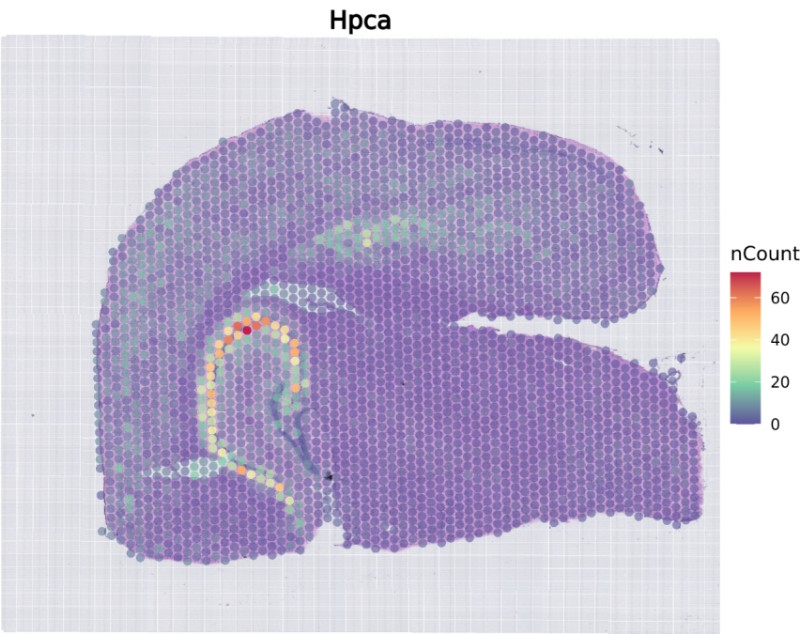
Hpca
Generate Cluster Plots for Specific Gene(s) with Dark Background
“`R
object <- Create_object(
FilePath = ‘E:/AAAWork/BSTViewer_project/subdata/L13_heAuto/’,
barcode_pos_file = ‘E:/AAAWork/BSTViewer_project/subdata/L13_heAuto/barcodes_pos.tsv.gz’,
out_path = ‘C:/Users/R/Desktop/temp/Test/Single_gene_2/’,
png_path = ‘C:/Users/R/Desktop/temp/he.png’,
point_size = 2.6, # Same as above.
Gene_stat = T, # Whether to generate marker gene plots (default: False).
Custom_gene = T, # Whether to perform custom gene plotting (default: False).
dark_background = T, # Use a dark background (default: False).
gene_list = c(‘Hpca’) # List of genes to plot, you can input multiple genes.
)
“`
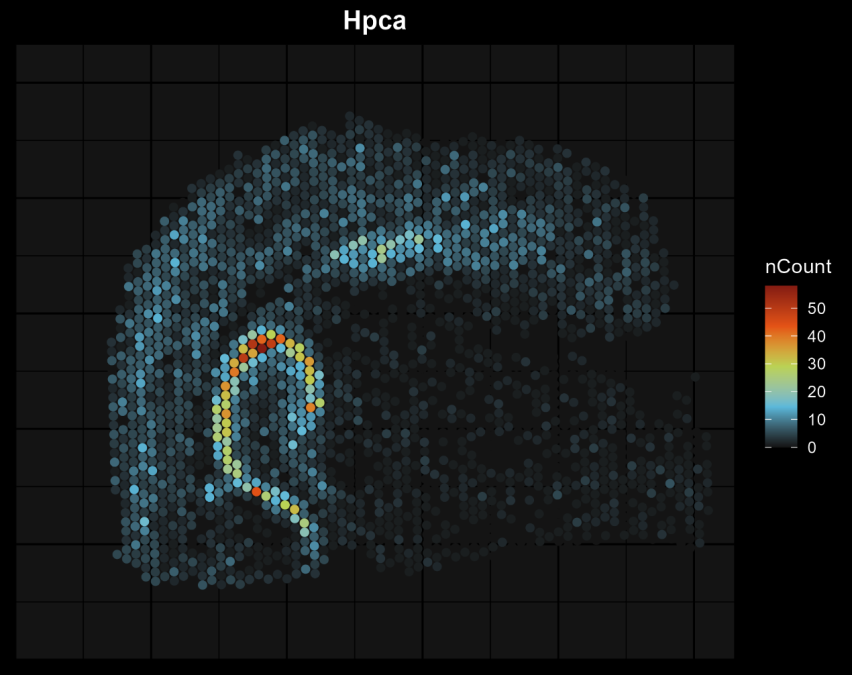
Hpca
- Generate a Clustering Plot for a Single Cluster
“`R
object <- Create_object(
FilePath = ‘E:/AAAWork/BSTViewer_project/subdata/L13_heAuto/’,
barcode_pos_file = ‘E:/AAAWork/BSTViewer_project/subdata/L13_heAuto/barcodes_pos.tsv.gz’,
out_path = ‘C:/Users/R/Desktop/temp/TestL6/single/’,
png_path = ‘C:/Users/R/Desktop/temp/he.png’,
point_size = 2, # Same as above.
Single_cluster = T # Whether to generate a clustering plot for a single cluster (default: False).
)
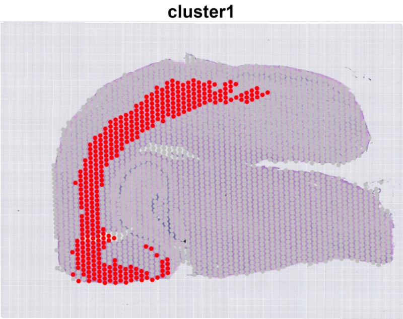
cluster1
Single cluster


 京公网安备 11011302003368号