细胞通讯分析流程与方法

细胞通讯分析流程与方法：细胞通讯分析的基础是基因表达数据和配体-受体数据库信息，例如转录组数据表明A、B细胞分别表达了基因α和β，通过数据库查询α和β是配体-受体关系，则认为A-B通过α-β途径进行了通讯。

输入数据格式要求：

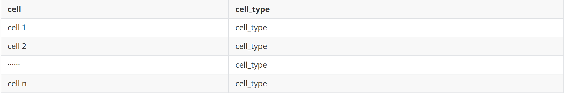
（1）细胞注释文件（meta.txt，两列，分别为细胞id和细胞类型）

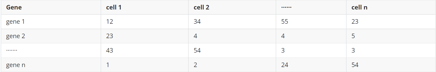
（2）基因表达矩阵（counts.txt）

#下载软件（按顺序安装）

conda create -n cellphonedb2 python=3.7

conda install Cython

conda install h5py

conda install scikit-learn

conda install r

conda install rpy2

pip install https://pypi.tuna.tsinghua.edu.cn/simple cellphonedb

pip install -i https://pypi.tuna.tsinghua.edu.cn/simple markupsafe==2.0.1

#R包

install.packages(‘ggplot2’)

install.packages(‘heatmap’)

#data1—> R

#使用RCTD注释的空间数据进行后续分析

results <- myRCTD@results

results_df <- results$results_df

barcodes = rownames(results_df[results_df$spot_class != “reject” & puck@nUMI >= 1,])

my_table = puck@coords[barcodes,]

my_table$class = results_df[barcodes,]$first_type

meta = my_table %>% select(class) %>% rownames_to_column(var = ‘cell’) %>% dplyr::rename(cell_type = class)

write.table(meta ,file = ‘/xxx/Test/meta.txt’, sep = ‘\t’, quote = F, row.names = T)

#data2—> R

expr <- Read10X(‘/xxx/BSTViewer_project/subdata/L13_heAuto/’,cell.column = 1)

object <- CreateSeuratObject(counts = expr,assay = “Spatial”)

counts = object[[‘Spatial’]]@counts %>% as.data.frame() %>% rownames_to_column(var = ‘Gene’)

write.table(counts ,file = ‘/xxx/Test/counts.txt’, sep = ‘\t’, quote = F, row.names = T)

#鼠源基因转化

#CellPhoneDB 只能识别人类基因，如果是鼠源基因需要进行同源基因的转化

#下载人鼠同源基因对应关系

http://asia.ensembl.org/biomart/martview/b9f8cc0248e4714ba8e0484f0cbe4f02

#细胞通讯分析流程与方法参考步骤

https://www.jianshu.com/p/922a7f2c21fc

#下载的对应关系表应该有四列

Gene_stable_ID  |   Gene_name   |   Mouse_gene_stable_ID    |   Mouse_gene_name

#将对应关系(human_mouse_gene.txt)替换到 data2 矩阵—>Shell

awk -F ‘\t’ ‘BEGIN{OFS == ‘\t’}ARGIND==1{a[$4]=$1}ARGIND==2{if(FNR ==1){print}else{$1 = a[$1];print}}’ human_mouse_gene.txt counts.txt | sed ‘/^ /d’ | sed ‘1s/^/Gene\t/’ | sed ‘s/\s/\t/g’ > counts_new.txt

#从远程存储库中列出cellphonedb可用数据库版本:

cellphonedb database list_remote

#查看本地数据库

cellphonedb database list_local

#下载远程数据库

cellphonedb database download –version <version_spec|latest>

#运行cellphonedb —> Shell

cellphonedb method statistical_analysis –output-path test_output meta.txt counts_new.txt

#输出文件

deconvoluted.txt    |   pvalues.txt |   significant_means.txt

test.count_network.txt  |   means.txt   |   test.interaction_count.txt

#气泡图—> Shell

cellphonedb plot dot_plot –pvalues-path test_output/pvalues.txt –means-path test_output/means.txt –output-path test_output  –output-name test.dotplot.pdf

#仅绘制自己关注的细胞和互作—> Shell

cellphonedb plot dot_plot –pvalues-path test_output/pvalues.txt –means-path test_output/means.txt –output-path test_output  –output-name test.dotplot2.pdf –rows test_output/row.txt –columns test_output/col.txt

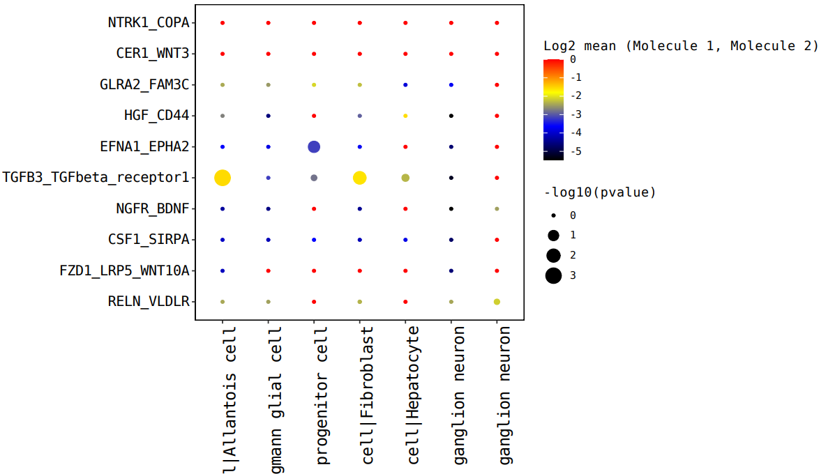
注：横坐标是细胞类型互作，纵坐标是蛋白互作，点越大表示 p 值越小，颜色代表平均表达量

#热图—> Shell

cellphonedb plot heatmap_plot –pvalues-path test_output/pvalues.txt –output-path test_output –pvalue 0.05 –count-name test.heatmap_count.pdf –log-name test.heatmap_log_count.pdf –count-network-name test.count_network.txt –interaction-count-name test.interaction_count.txt meta.txt

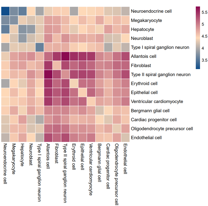
注：横纵坐标表示细胞类型，颜色深蓝色到紫红色代表互作数由低到高

#细胞通讯分析流程与方法：细胞类型网络图—> R

#这里借用另一款细胞通讯分析软件——CellChat(https://github.com/sqjin/CellChat)的绘图方法

#加载R包

library(igraph)

library(tidyr)

library(stats)

library(reshape2)

library(Matrix)

library(grDevices)

library(ggplot2)

#使用CellChat作者提供的绘制互作网络图的function

scPalette <- function(n) {

colorSpace <- c(‘#E41A1C’,’#377EB8′,’#4DAF4A’,’#984EA3′,’#F29403′,’#F781BF’,’#BC9DCC’,’#A65628′,’#54B0E4′,’#222F75′,’#1B9E77′,’#B2DF8A’,

‘#E3BE00′,’#FB9A99′,’#E7298A’,’#910241′,’#00CDD1′,’#A6CEE3′,’#CE1261′,’#5E4FA2′,’#8CA77B’,’#00441B’,’#DEDC00′,’#B3DE69′,’#8DD3C7′,’#999999′)

if (n <= length(colorSpace)) {

colors <- colorSpace[1:n]

} else {

colors <- grDevices::colorRampPalette(colorSpace)(n)

}

return(colors)

}

netVisual_circle <-function(net, color.use = NULL,title.name = NULL, sources.use = NULL, targets.use = NULL, idents.use = NULL, remove.isolate = FALSE, top = 1,

weight.scale = FALSE, vertex.weight = 20, vertex.weight.max = NULL, vertex.size.max = NULL, vertex.label.cex=1,vertex.label.color= “black”,

edge.weight.max = NULL, edge.width.max=8, alpha.edge = 0.6, label.edge = FALSE,edge.label.color=’black’,edge.label.cex=0.8,

edge.curved=0.2,shape=’circle’,layout=in_circle(), margin=0.2, vertex.size = NULL,

arrow.width=1,arrow.size = 0.2){

if (!is.null(vertex.size)) {

warning(“‘vertex.size’ is deprecated. Use `vertex.weight`”)

}

if (is.null(vertex.size.max)) {

if (length(unique(vertex.weight)) == 1) {

vertex.size.max <- 5

} else {

vertex.size.max <- 15

}

}

options(warn = -1)

thresh <- stats::quantile(net, probs = 1-top)

net[net < thresh] <- 0

if ((!is.null(sources.use)) | (!is.null(targets.use)) | (!is.null(idents.use)) ) {

if (is.null(rownames(net))) {

stop(“The input weighted matrix should have rownames!”)

}

cells.level <- rownames(net)

df.net <- reshape2::melt(net, value.name = “value”)

colnames(df.net)[1:2] <- c(“source”,”target”)

# keep the interactions associated with sources and targets of interest

if (!is.null(sources.use)){

if (is.numeric(sources.use)) {

sources.use <- cells.level[sources.use]

}

df.net <- subset(df.net, source %in% sources.use)

}

if (!is.null(targets.use)){

if (is.numeric(targets.use)) {

targets.use <- cells.level[targets.use]

}

df.net <- subset(df.net, target %in% targets.use)

}

if (!is.null(idents.use)) {

if (is.numeric(idents.use)) {

idents.use <- cells.level[idents.use]

}

df.net <- filter(df.net, (source %in% idents.use) | (target %in% idents.use))

}

df.net$source <- factor(df.net$source, levels = cells.level)

df.net$target <- factor(df.net$target, levels = cells.level)

df.net$value[is.na(df.net$value)] <- 0

net <- tapply(df.net[[“value”]], list(df.net[[“source”]], df.net[[“target”]]), sum)

}

net[is.na(net)] <- 0

if (remove.isolate) {

idx1 <- which(Matrix::rowSums(net) == 0)

idx2 <- which(Matrix::colSums(net) == 0)

idx <- intersect(idx1, idx2)

net <- net[-idx, ]

net <- net[, -idx]

}

g <- graph_from_adjacency_matrix(net, mode = “directed”, weighted = T)

edge.start <- igraph::ends(g, es=igraph::E(g), names=FALSE)

coords<-layout_(g,layout)

if(nrow(coords)!=1){

coords_scale=scale(coords)

}else{

coords_scale<-coords

}

if (is.null(color.use)) {

color.use = scPalette(length(igraph::V(g)))

}

if (is.null(vertex.weight.max)) {

vertex.weight.max <- max(vertex.weight)

}

vertex.weight <- vertex.weight/vertex.weight.max*vertex.size.max+5

loop.angle<-ifelse(coords_scale[igraph::V(g),1]>0,-atan(coords_scale[igraph::V(g),2]/coords_scale[igraph::V(g),1]),pi-atan(coords_scale[igraph::V(g),2]/coords_scale[igraph::V(g),1]))

igraph::V(g)$size<-vertex.weight

igraph::V(g)$color<-color.use[igraph::V(g)]

igraph::V(g)$frame.color <- color.use[igraph::V(g)]

igraph::V(g)$label.color <- vertex.label.color

igraph::V(g)$label.cex<-vertex.label.cex

if(label.edge){

igraph::E(g)$label<-igraph::E(g)$weight

igraph::E(g)$label <- round(igraph::E(g)$label, digits = 1)

}

if (is.null(edge.weight.max)) {

edge.weight.max <- max(igraph::E(g)$weight)

}

if (weight.scale == TRUE) {

#E(g)$width<-0.3+edge.width.max/(max(E(g)$weight)-min(E(g)$weight))*(E(g)$weight-min(E(g)$weight))

igraph::E(g)$width<- 0.3+igraph::E(g)$weight/edge.weight.max*edge.width.max

}else{

igraph::E(g)$width<-0.3+edge.width.max*igraph::E(g)$weight

}

igraph::E(g)$arrow.width<-arrow.width

igraph::E(g)$arrow.size<-arrow.size

igraph::E(g)$label.color<-edge.label.color

igraph::E(g)$label.cex<-edge.label.cex

igraph::E(g)$color<- grDevices::adjustcolor(igraph::V(g)$color[edge.start[,1]],alpha.edge)

if(sum(edge.start[,2]==edge.start[,1])!=0){

igraph::E(g)$loop.angle[which(edge.start[,2]==edge.start[,1])]<-loop.angle[edge.start[which(edge.start[,2]==edge.start[,1]),1]]

}

radian.rescale <- function(x, start=0, direction=1) {

c.rotate <- function(x) (x + start) %% (2 * pi) * direction

c.rotate(scales::rescale(x, c(0, 2 * pi), range(x)))

}

label.locs <- radian.rescale(x=1:length(igraph::V(g)), direction=-1, start=0)

label.dist <- vertex.weight/max(vertex.weight)+2

plot(g,edge.curved=edge.curved,vertex.shape=shape,layout=coords_scale,margin=margin, vertex.label.dist=label.dist,

vertex.label.degree=label.locs, vertex.label.family=”Helvetica”, edge.label.family=”Helvetica”) # “sans”

if (!is.null(title.name)) {

text(0,1.5,title.name, cex = 1.1)

}

# https://www.andrewheiss.com/blog/2016/12/08/save-base-graphics-as-pseudo-objects-in-r/

# grid.echo()

# gg <-  grid.grab()

gg <- recordPlot()

return(gg)

}

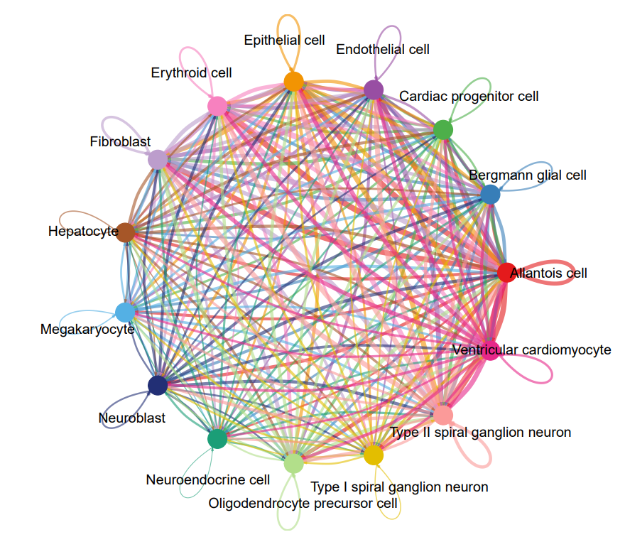
#整体互作网络图绘制

#读取cellphonedb的分析数据

count_net <- read.delim(“/xxx/test_output/test.count_network.txt”, check.names = FALSE)

#数据格式处理

count_inter <- count_net

count_inter$count <- count_inter$count/100

count_inter <- spread(count_inter, TARGET, count)

rownames(count_inter) <- count_inter$SOURCE

count_inter <- count_inter[, -1]

count_inter <- as.matrix(count_inter)

#绘图

netVisual_circle(count_inter,weight.scale = T)

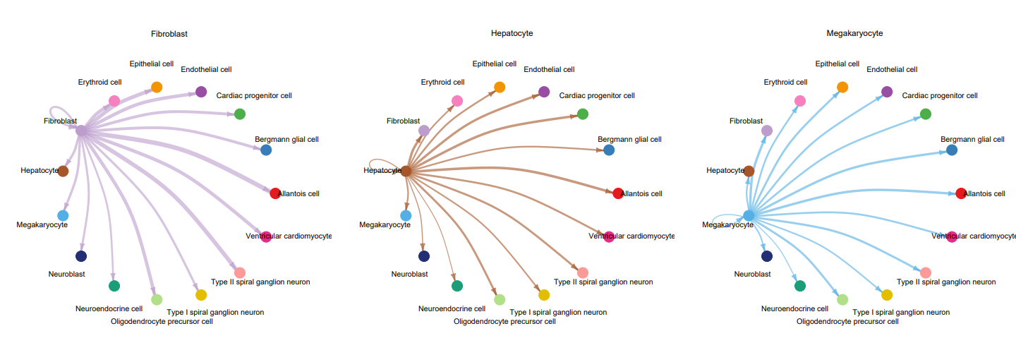
#细胞通讯分析流程与方法：每种细胞与其他细胞的互作

par(mfrow = c(1,3), xpd=TRUE)

for (i in 1:nrow(count_inter)) {

mat2 <- matrix(0, nrow = nrow(count_inter), ncol = ncol(count_inter), dimnames = dimnames(count_inter))

mat2[i, ] <- count_inter[i, ]

netVisual_circle(mat2,

weight.scale = T,

edge.weight.max = max(count_inter),

title.name = rownames(count_inter)[i],

arrow.size=0.2)

}