monocle 分析之细胞聚类

安装monocle 包

monocle 分析之数据导入

monocle 分析之细胞聚类

数据预处理降维、可视化

去批次效应后重新降维

monocle3可以分析大型、复杂的单细胞数据，可处理数百万个细胞。monocle3主要更新了哪些功能？

1.一个更好的结构化工作流程来学习发展轨迹。

2.支持 UMAP 算法初始化轨迹推断。

3.支持具有多个root的轨迹。

4.学习具有循环或收敛点的轨迹的方法(Ways to learn trajectories that have loops or points of convergence)。

5.利用“近似图抽象”的思想，⾃动划分细胞以学习不相交或平⾏轨迹的算法。

6.一种新的对轨迹依赖表达的基因的统计测试。这将替换旧的differalgenetest()函数和BEAM()。

7.3D界面可视化轨迹和基因表达。

安装monocle3包

要求R > 3.6.1

1、安装Bioconductor

1 if (!requireNamespace(“BiocManager”, quietly = TRUE))

2 install.packages(“BiocManager”)

3 BiocManager::install(version = “3.10”)

2、安装依赖包

1 BiocManager::install(c(‘BiocGenerics’, ‘DelayedArray’, ‘DelayedMatrixStats’,

2 ‘limma’, ‘S4Vectors’, ‘SingleCellExperiment’,

3 ‘SummarizedExperiment’, ‘batchelor’, ‘Matrix.utils’))

3、安装monocle3

1 install.packages(“devtools”)

2 devtools::install_github(‘cole-trapnell-lab/leidenbase’)

3 devtools::install_github(‘cole-trapnell-lab/monocle3’)

如果不能联网下载，可以下载到本地然后本地安装

1 library(devtools)

2 install_local(“D:/monocle3-0.2.2.tar.gz”)

monocle3分析之数据导入

1、从seurat对象生成 cell_data_set （CDS）对象

.expression_matrix , a numeric matrix of expression values, where rows are genes, and columns are cells

.cell_metadata , a data frame, where rows are cells, and columns are cell attributes (such as cell type, culture condition, day captured, etc.)

.gene_metadata , an data frame, where rows are features (e.g. genes), and columns are gene attributes, such as biotype, gc content, etc.

注：表达矩阵的⾏数必须与gene_metadata相同，表达矩阵的列必须与cell_metadata相同

1 library(monocle3)

2 sceObj <- readRDS(“/path/sce_test.Rds”)

3 expression <- GetAssayData(sceObj, assay = ‘RNA’, slot = ‘counts’)

4 cell_metadata <- sceObj@meta.data

5 gene_annotation <- data.frame(gene_short_name = rownames(expression))

6 rownames(gene_annotation) <- rownames(expression)

7 monocle_cds <- new_cell_data_set(expression, cell_metadata = cell_metadata, gene_metadata = gene_annotation)

2、直接从10X cellranger生成CDS对象

monocle_cds 注：也可以使⽤ load_mm_data() 函数读取 MatrixMarket 格式数据

monocle3分析之细胞聚类

我们使用monocle3对数据进行聚类分析。

数据预处理

使用 preprocess_cds 对数据进行normalize 以及 PCA 降维

monocle_cds <- preprocess_cds(monocle_cds, num_dim = 50)

注：可以使⽤ plot_pc_variance_explained() 函数画肘部图，从中选择合适的 PCs 数降维、可视化

1 monocle_cds <- reduce_dimension(monocle_cds, preprocess_method = “PCA”) # 默认使⽤UMAP

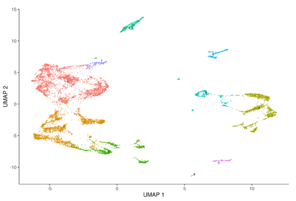
2 plot_cells(monocle_cds, color_cells_by=”seurat_clusters”) # umap显示原seurat 细胞聚类的结果
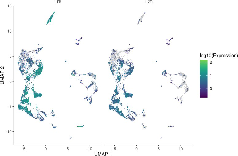
 plot_cells(monocle_cds, genes=c(“LTB”, “IL7R”)) # 显示某几个基因的表达

去批次效应后重新降维
检查样本间批次效应

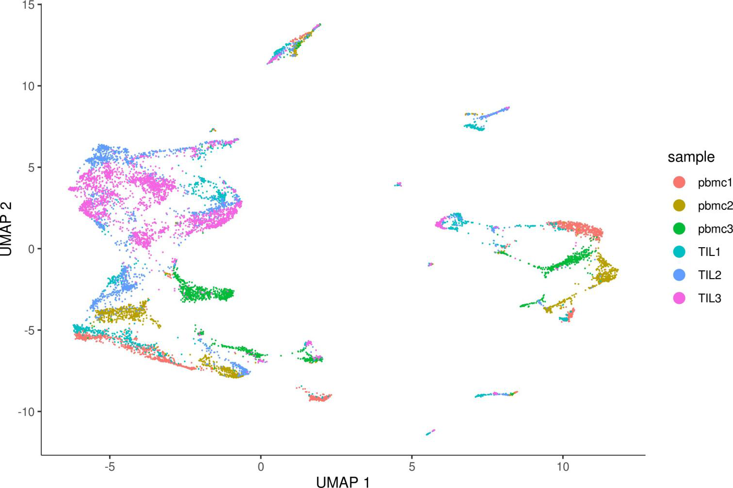
plot_cells(monocle_cds, color_cells_by=”sample”, label_cell_groups=FALSE) # 检查样本间的批次效应
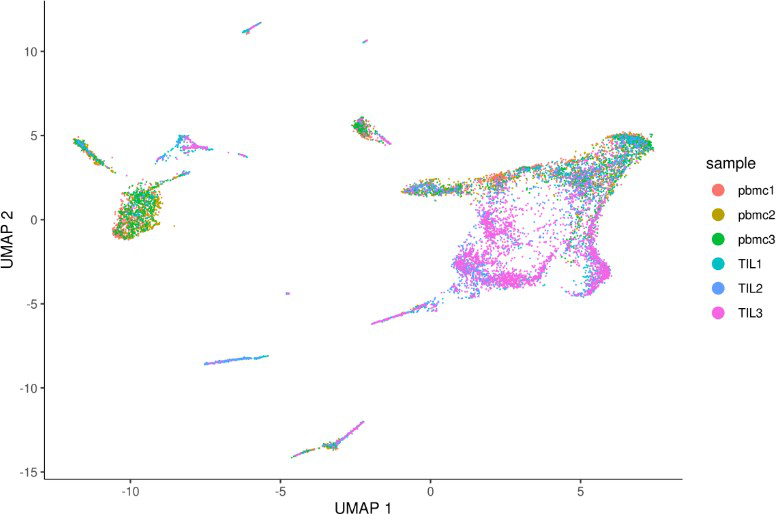
align_cds移除批次效应
1 # align_cds() tries to remove batch effects using mutual nearest neighbor alignment
2 monocle_cds <- align_cds(monocle_cds, num_dim = 100, alignment_group = “sample”) # 去除批次效应,似乎不太好使
3 monocle_cds <- reduce_dimension(monocle_cds)
plot_cells(monocle_cds, color_cells_by=”sample”, label_cell_groups=FALSE)

细胞聚类
1 # monocle3同样可以指定resolution（默认NULL），但需要注意，resolution 设置⽐ seurat⼩很多（例如当resolution=0.1时，出现⼏百个cluster）
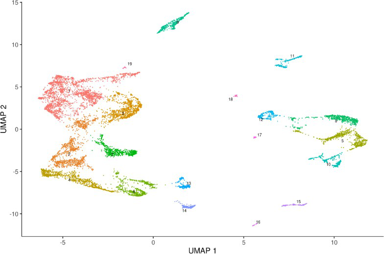
2 monocle_cds <- cluster_cells(monocle_cds, resolution = 0.0001, reduction_method = “umap”)
3 plot_cells(monocle_cds)

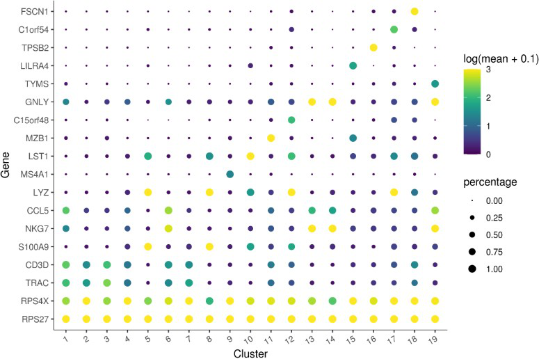
Marker 基因分析
使用 top_markers() 函数寻找cluster之间的marker基因。
1# 可以选择 cluster 也可以选择 partitions
2as.character(partitions(monocle_cds)) %>% unique
3 [1] “3” “2” “6” “11” “4” “7” “1” “5” “9” “10” “8”
4 as.character(clusters(monocle_cds)) %>% unique
5 [1] “8” “4” “10” “14” “19” “9” “15” “2” “7” “1” “6” “5” “13” “11”
“17”
6 [16] “3” “12” “18” “16”
7
8marker_test_res 9head(marker_test_res, n = 3)
10gene_id gene_short_name cell_group marker_score mean_expression 11 1 HES4 HES4 10 0.2511486 0.9178898
12 2 TNFRSF18 TNFRSF18 3 0.2701016 3.8953993
13 3 TNFRSF4 TNFRSF4 3 0.3305234 5.8852331
14 fraction_expressing specificity pseudo_R2 marker_test_p_value 15 1 0.6170213 0.4070340 0.3236830 4.873175e-105 16 2 0.7234243 0.3733654 0.2931210 9.156877e-159 17 3 0.7102540 0.4653594 0.3062058 5.322088e-166
18 marker_test_q_value 19 1 1.317746e-99
20 2 2.476093e-153
21 3 1.439135e-160
22marker_test_res 23top_specific_markers %
24filter(fraction_expressing >= 0.10) %>%
25group_by(cell_group) %>%
26top_n(1, pseudo_R2)
27top_specific_marker_ids % pull(gene_id))
28plot_genes_by_group(monocle_cds,
29top_specific_marker_ids,
30group_cells_by=”cluster”,
31ordering_type=”maximal_on_diag”,
max.size=3
1 # 将monocle3结果存到seurat对象中
2 colData(monocle_cds)$monocle3_partitions <- as.character(partitions(monocle_cds))
3 colData(monocle_cds)$monocle3_clusters <- as.character(clusters(monocle_cds))
4 sceObj@meta.data <- pData(monocle_cds) %>% as.data.frame

百迈客不仅提供标准分析内容，还提供个性化分析内容，全新的monocle3 数据分析，详情可见单细胞转录组分析难？教您2步，轻松玩转它。更多好玩的，生信分析内容尽在百迈客云平台，如果感兴趣欢迎点击按钮联系我们，我们将免费为您设计文章思路分析方案。